Doing distributed data analysis on a Raspberry Pi cluster
Thu Sep 12 2019tags: programming build making data science internship inzura apache spark GIS scala raspberry pi minio public project featured
(Summer 2019 internship with Inzura)
This is the second project I've done with Raspberry Pis. The first one was a Raspberry Pi game console done back in 2017.
As far as I know, this is the largest Apache Spark Raspi cluster that has been published online. There's an eight-node Raspi 4 cluster here and a six-node Raspi 2 cluster here but i) ours is the biggest and ii) we have actually used the cluster to do "real" data analysis.
Results
I calculated average traffic speeds of a sample of 50,000 trips in the UK. These trips were recorded from drivers who used Inzura's mobile app. The vast majority of trips were in Northern Ireland, and I've chosen to zoom in on the traffic data in Belfast, Northern Ireland. These are chloropleth maps: roads with low average speeds are dark purple, and roads with high average speeds bright yellow.
This is a really high-resolution image, best opened and viewed in full-size. It shows the extent of coverage of the trips that I sampled. We can see that while the data covers the entirety of the UK, most of the trips are from Northern Ireland (NI).
As we zoom into NI we see that almost the entire landmass has been traversed. We can clearly make out city centers, and the roads that connect them: Belfast is by far the largest and most prominent---although one can make out other cities like Bangor and Lisburn near it. We can also see Donegal and Omagh in the west.
We can glean some insights even at this distance. We can see that average speeds in cities tend to be low (dark purple), while roads that connect cities have higher average speeds.
Let's zoom in a little:
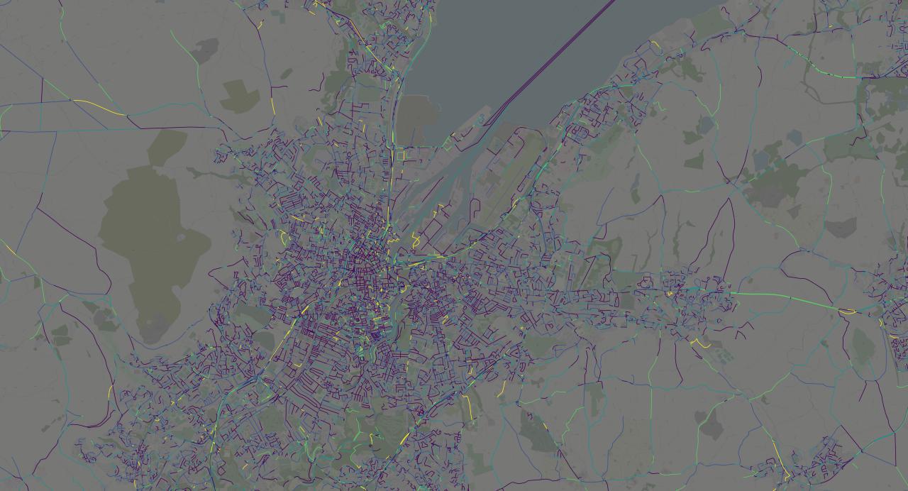
We can now clearly see the shape of Belfast and the cities near it. There's an interesting funnel shape at the top, almost like it's feeding into Belfast proper. There's also what looks like extensions of the city to the south-west: are these part of Belfast too, or cities in their own right?
From the road network alone we can see that towns usually set up near the coast: the road network on both sides of the bay is much denser than bits closer inland.
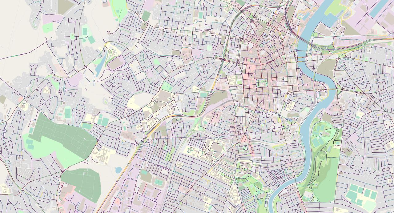
Now let's zoom in to Belfast proper:
At this zoom level the layout of the city can clearly be discerned. Streets near the center of the city are laid out in a neat and densely-packed grid pattern, which gives way to a sparser, more organic layout toward the
We can even see some ferry routes from the pier! These are routes to the mainland and the Isle of Man.
Most interestingly, we can see an S-shaped road that snakes through the city. It starts from the southwest and winds its way up northeast. We can see that it is a different colour from the rest of the city's roads, which are mostly dark purple: this road has segments of yellow and green.
Here's the same image with the background darkened so we can see the colours more clearly:
We can really make out the S-shaped road here, and a couple more besides. There's a road leading down from the northeast that looks like a main connection to the northeastern coast.
One final zoom in to 1:25000 scale:
The shape (and colour) of the S-shaped road is apparent now.
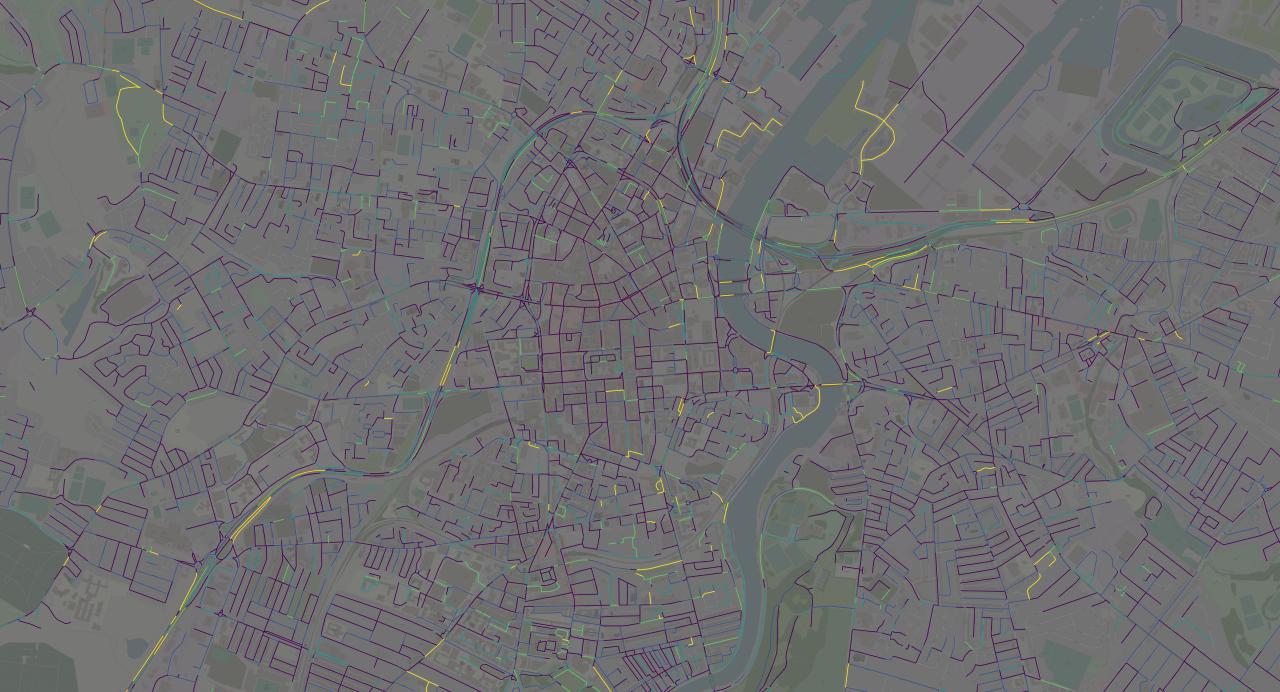
Average speeds on the S-shaped road decrease when there is a bend in the road, and when there is an intersection. Notice also that roads on the periphery tend to have higher average velocities, although this could be because there is not enough data on them (thus throwing off the averages).
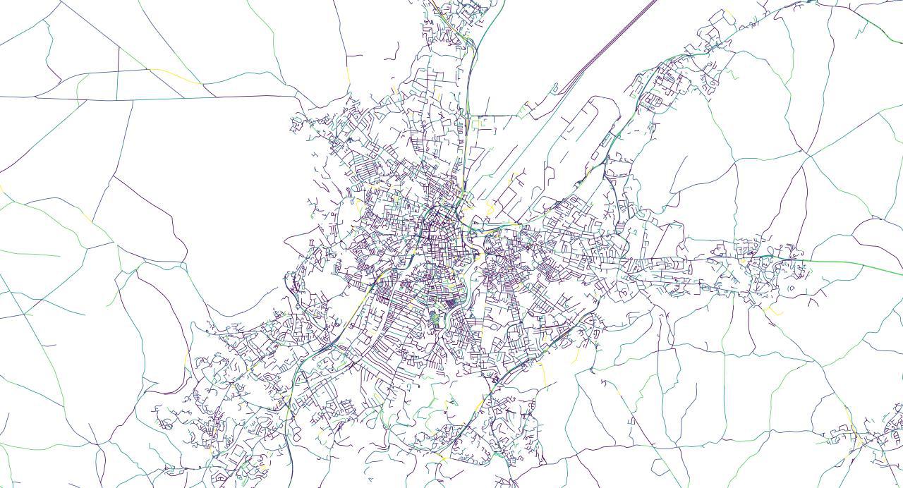
One final render without the background---just because it looks pretty, and shows us the shape of the city:
Raspberry Pi compute cluster
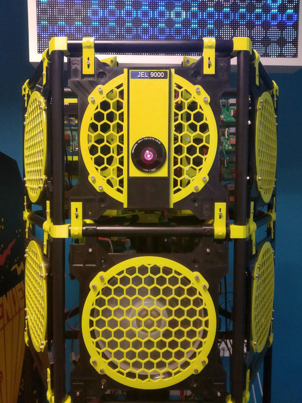
This is the Raspberry Pi compute cluster. It's taller than a man:
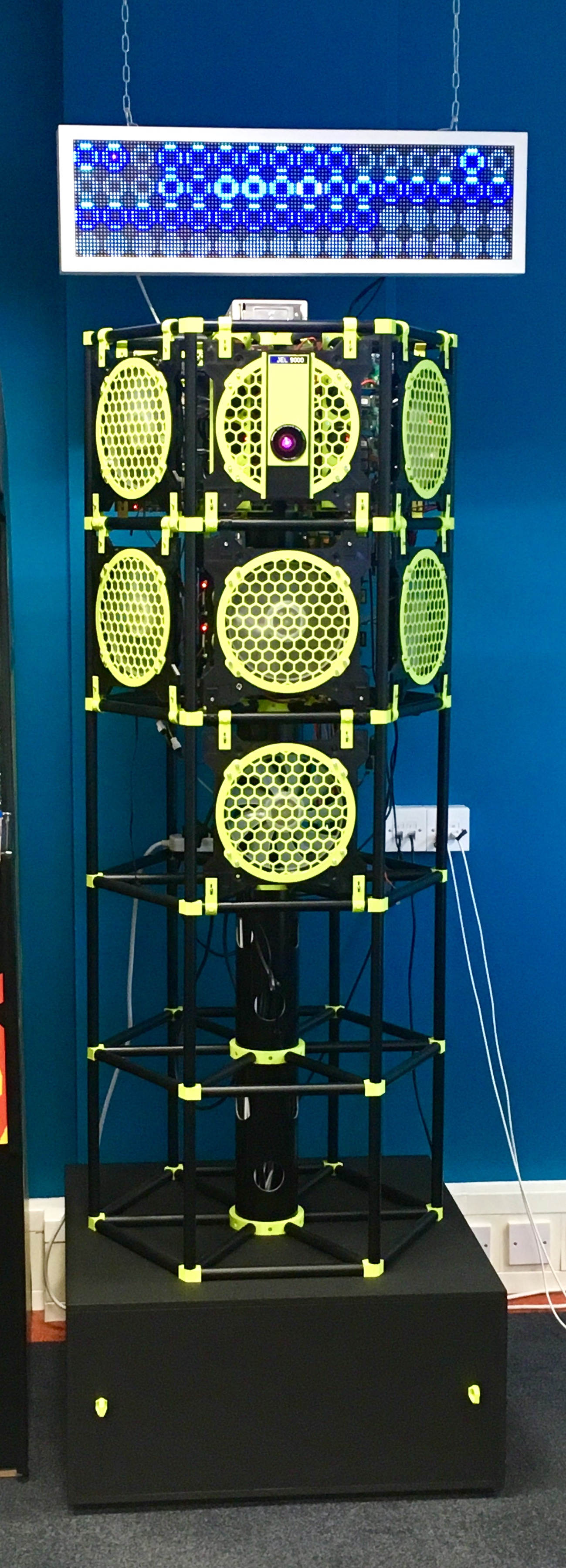
It was designed and built by Richard Jelbert, the CEO and co-founder of Inzura. Almost everything you see is 3D-printed: that includes the faceplates, the clips and the holding rack (for the Raspis). It contains 16 Raspi 4s and 25 assorted Raspi 3B/3/2/1s. For this project I only used the Raspi 4s.
The structure of the cluster is hexagonal: there are 5 storeys and 6 segments on each storey. One of the segments is reserved for SSDs (data storage and database lookups), but the other 5 segments can be used for compute.
I'm sorry Dave, I'm afraid I can't do that
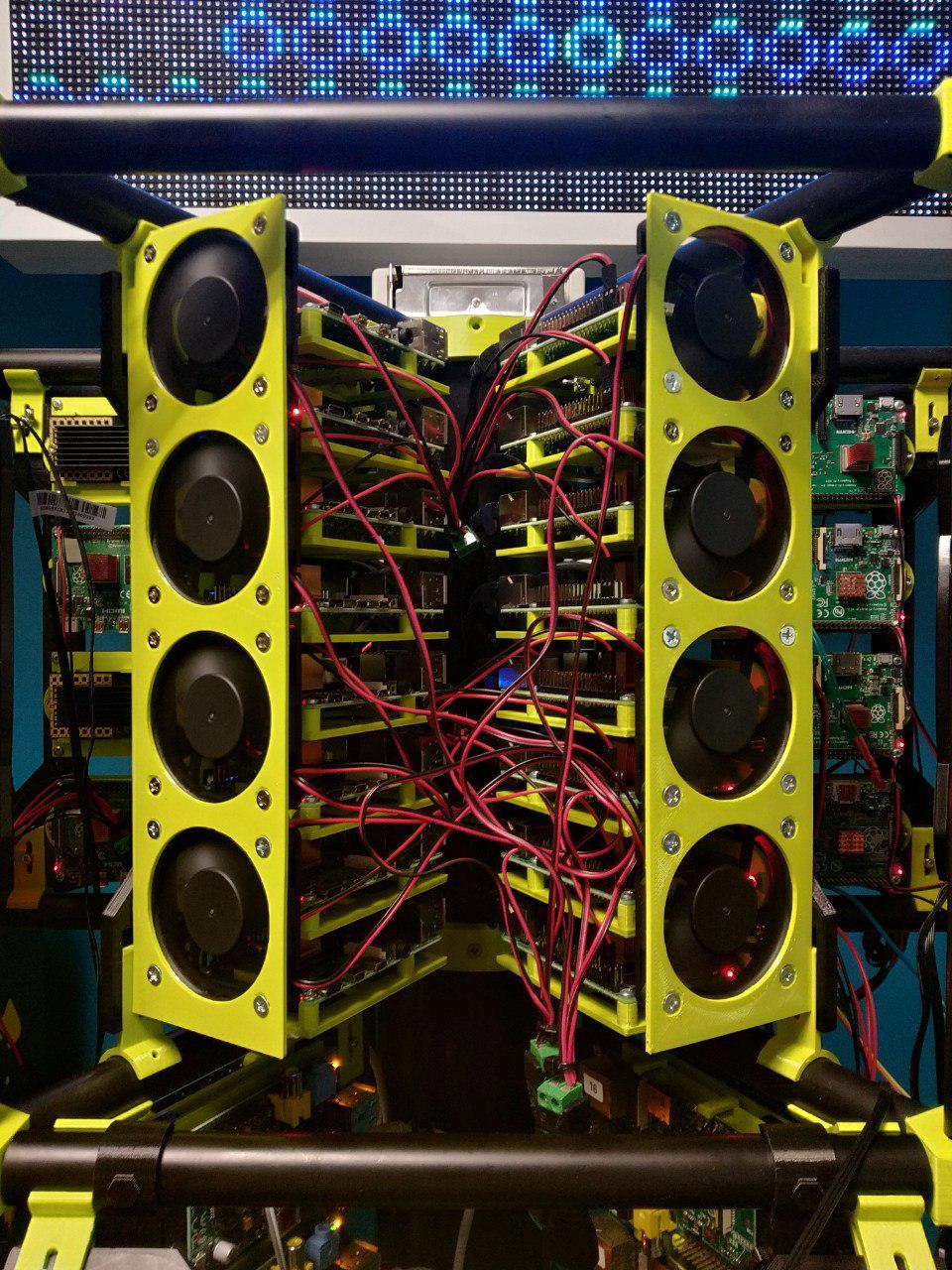
The front panel opens up to expose the internals:
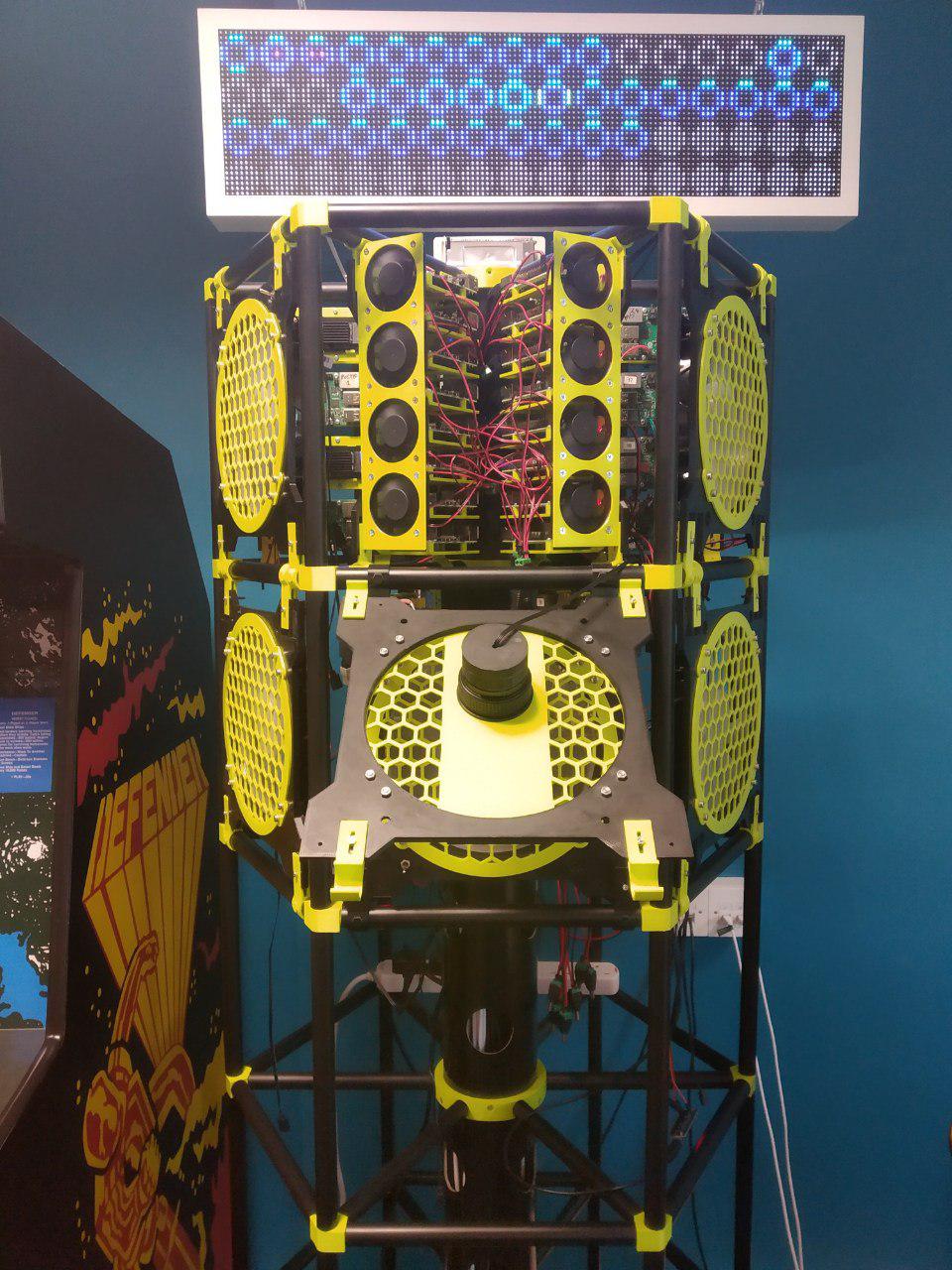
Again, all of this is 3D-printed. 8 Raspberry Pi 4s sit on each rack and are cooled by 4 mini-fans per rack (the cooling is necessary to prevent them throttling).
The cluster has a theoretical maximum capacity of 400 Raspis (16 Raspis per segment, 5 segments per storey, 5 storeys total); Richard said that cooling may be tricky at that density, but 12 Raspis per segment is definitely doable. That gives us an actual capacity of 300 Raspis in the cluster.
It is also possible to cluster MinIO across up to 16 nodes. Minio allows distributed object storage: it lets my code run without having a copy of every single file on every single Raspi. Given that we need only 1 SSD per storey, this will be sufficient for our purposes.
Why use the cluster?
Why go to all the trouble to set up a compute cluster? Why not run it on a single machine?
- It's the only scalable solution when the number of trips gets large
- We get increased performance by parallelising computation
- It's cool!
Scalability
I had only been able to download a small sample of 50,000 anonymised trips. But Inzura has a corpus of millions of trips and growing. It certainly doesn't fit on a single machine's memory (it doesn't even fit on disk). So the most naive approach of reading all the files into memory at once and calculating the average that way won't work. Something that does work is to read the files in one by one and calculate the averages that way, but this is of course rather slow. Which leads us to ...
Performance
The task is to calculate average road speed for every road in the database. This is an embarassingly parallelisable task: each trip is an individual JSON file (which means we don't have to worry about shared memory), and there is almost no work needed to combine the results of disparate parallel computations. This means that we can get a close-to-linear speedup simply by adding more computers --- which means that a cluster of Raspberry Pis will outperform even a beefy (and much more expensive) computer.
Even if 16 Raspis don't outperform a single computer, 300 Raspis certainly will, and it is easy now to add more Raspis now that the groundwork has been laid. This opens the door to all sorts of future data analysis and exploration tasks which may be prohibitively expensive for a single computer to run (in terms of wall-clock time).
Cool factor
Why not just use Google Cloud or something?---because this is cooler and more educational.
Configuring the cluster
Configuring the cluster was by far the hardest part of this project. Any instructions I could find for setting up a Spark cluster were either incomplete, out of date, or incorrect. It took Richard, Chris and I three full days to set everything up. Eventually I heavily modified this MinIO cookbook and successfully deployed Spark on the 16 worker Raspis:
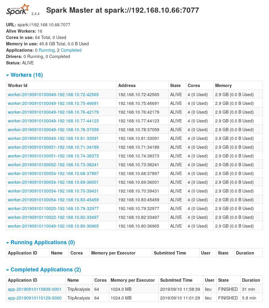
The cluster computer has 64 cores and 64GB of memory (45GB free)---already much better than my laptop.
I have written a bash script that should automate (but not completely) the
installation process
here.
The only thing one has to do apart from this is to edit the core-site.xml
file to point to one's S3 bucket/MinIO server.
Apache Spark code
I gained the necessary knowledge to do this data analysis project by working through part of the Functional Programming in Scala Specialisation. I finished the courses Functional Programming Principles in Scala, Parallel Programming and Big Data Analysis with Scala and Spark. The last course was the most directly relevant to this project but I found the first course incredibly helpful for learning Scala (and the functional programming paradigm), and the third course for reasoning about parallel programs. Both courses helped me appreciate why Scala is a good language for data analysis---many of the functional abstractions of mapping over an iterable of some sort carry over almost directly to distributed computing.
I found Spark quite concise, although the documentation was quite lacking. Nonetheless, I was able to write the program in only about 20 lines of code.
The code does the following:
- Read a JSON file onto the Raspi
- Extract all the roads and velocities from the JSON file (Map step)
- Combine all the roads and find the average velocities from all the JSON files (Reduce step)
- Saves it into a single CSV file (the
coalescestep). This step is optional (and in fact is probably not recommended when the data set gets larger). I did it to make it easier to visualise in QGIS.
In total there were 50,000 trips, ~85 million data points, and ~170,000 unique road IDs.
object SimpleApp {
  def main(args: Array[String]) {
    import org.apache.spark.sql.SparkSession
    import org.apache.spark.sql.functions.explode
    val spark = SparkSession.builder.appName("TripAnalysis").getOrCreate()
    import spark.implicits._
    val results_path = "s3a://results/"
    val paths = "s3a://trips/*"
    val tripDF = spark.read.option("multiline", "true").json(paths)
	// "Explode" the data array into individual rows
    val linksDF = tripDF.select(explode($"data").as("data"))
    val linksDF2 = linksDF.select("data.dbResponse.linkID", "data.absVelocity")
    // create a temporary view using the DataFrame
    linksDF2.createOrReplaceTempView("times")
    /*
      root
      |-- linkID: string (nullable = true)
      |-- absVelocity: double (nullable = true)
    */
    val tDF = spark.sql("SELECT CAST(linkID as LONG), absVelocity from times
	WHERE linkID IS NOT NULL AND absVelocity IS NOT NULL")
    val groupedDS = tDF.groupBy("linkID")
    val avgsDS = groupedDS.agg(
      "linkID" -> "count",
      "absVelocity" -> "avg"
    ).sort($"linkID".asc)

    avgsDS.coalesce(1).write.
    option("header", "true").
    csv(results_path + "results_49998")
    spark.stop()
  }
}
The Spark code gives the road IDs, but we still have to get the coordinates that that road ID corresponds to. So I queried the road database (which also runs in the cluster) with a couple of lines of throwaway Python code.
I had written a SQL utility function for my previous project on optimising SMS messages which I was able to reuse here.
import time
from sql_utils import query

# First read csv

import csv

rows = []

with open("results-49998.csv") as f:
    csvreader = csv.reader(f)
    header = next(csvreader, None)
    print(header)
    for row in csvreader:
        rows.append(row)

BATCH_SIZE = 10000
NUM_ROWS = len(rows)

pointer = 0

# Break up the rows

link_ids = [x[0] for x in rows]

all_start = time.time()
while pointer < NUM_ROWS:
    start = time.time()
    link_ids_subset = link_ids[pointer:pointer+BATCH_SIZE]
    array_string = ", ".join(str(i) for i in link_ids_subset)
    array_string = f"({array_string})"
    query_string = f"SELECT geom from (SELECT DISTINCT(link_id), " +
	"geom FROM streets WHERE link_id IN {array_string}) as f"

    # Send out the query
    query_result = (query(query_string))
    for i in range(pointer, min(pointer+BATCH_SIZE, len(rows))):
        rows[i].append(query_result[i-pointer][0])

    end = time.time()
    print(f"Time taken to do {pointer}:{pointer+BATCH_SIZE}: {end-start}")

    pointer += BATCH_SIZE

all_end = time.time()

print(f"Time taken to make all the queries: {all_end-all_start}")

header.append("geom")

with open("results-49998-with-geom.csv", "w") as f:
    f.write(",".join(str(i) for i in header))
    f.write('\n')

with open("results-49998-with-geom.csv", "a") as f:
    for row in rows[:NUM_ROWS]:
        f.write(",".join(str(i) for i in row))
        f.write('\n')
There are issues with such an approach: when the number of unique road IDs get large, we won't be able to load all the rows into memory like I do here. But there were only ~140,000 unique link IDs, and I think even if you were to cover the whole of the UK the number of links would not exceed 2 million --- which fits well within the memory of a single machine.
I made two main optimisations.
First of all, I batched up the queries (instead of querying SELECT * FROM streets WHERE link_ID = linkid, do WHERE link_ID IN {array_string}) because
I knew that latency would be the primary bottleneck. This gave a huge speedup:
making 10,000 queries (without caching) only took about 1.2 seconds. To give a
comparison, measured round-trip time was about 0.1s (100ms); if I had made
140,000 individual queries, this would have taken 14,000 seconds (4 hours!),
and I was able to do all the queries in 14 seconds.
Second, I knew that the linkIDs were indexed in the database, and so I made sure to sort the linkIDs before batching and sending them to maximise the probability of a cache hit.
(base) lieu@bigbeast:~/dev/cluster-computing$ python3 get_road_geom.py
['linkID', 'count(linkID)', 'avg(absVelocity)']
Time taken to do 0:10000: 0.5610289573669434
Time taken to do 10000:20000: 0.48032593727111816
Time taken to do 20000:30000: 0.5004429817199707
Time taken to do 30000:40000: 0.5266928672790527
Time taken to do 40000:50000: 0.5340712070465088
Time taken to do 50000:60000: 0.6023671627044678
Time taken to do 60000:70000: 0.5589091777801514
Time taken to do 70000:80000: 0.48449015617370605
Time taken to do 80000:90000: 0.543027400970459
Time taken to do 90000:100000: 0.5296523571014404
Time taken to do 100000:110000: 0.6949601173400879
Time taken to do 110000:120000: 1.437162160873413
Time taken to do 120000:130000: 1.2379283905029297
Time taken to do 130000:140000: 1.15696120262146
Time taken to make all the queries: 9.848754644393921
The final CSV looked like this:
linkID;count(linkID);avg(absVelocity);geom
17341260;3;25.53091932029027;LINESTRING (-4.17935 53.21241, -4.17968 53.21257, -4.18033 53.21294, -4.18115 53.21319, -4.18138 53.2133, -4.18184 53.21339, -4.18204 53.21346, -4.18262 53.21369, -4.18334 53.21389, -4.18394 53.21439, -4.18473 53.21465, -4.18535 53.21475, -4.18618 53.21478)
17341303;1;31.053999640650744;LINESTRING (-4.17386 53.2051, -4.17501 53.20569, -4.17523 53.2058, -4.17534 53.20584)
The LINESTRING is a Well-Known Text (WKT) geometry representation and corresponds to the coordinates that a road occupies.
Future extensions
Now that the groundwork is done, future extensions become merely an issue of writing new code in Spark (which is, IMO, the easiest part). Some very nice and (relatively) low-hanging fruit to pluck include:
- Subdividing average speeds by time of day (so we can see how traffic conditions vary with time). We can even do a nice animation.
- Bringing in the full database of millions of anonymised trips in the corpus (possibly by connecting directly to the AWS servers rather than using a local MinIO instance)
Additionally, we can use the calculated average speeds to give a more personalised metric of driver safety. At the moment, a driver's score is determined (in part) by whether or not he drives over the speed limit of a road. But many roads do not fit their posted speed limits. It would be more enlightening to compare a driver's driving patterns to a reference distribution of other drivers on the same roads---and this data analysis helps us create that reference distribution.
Finally, we could use the ground truth of average speeds as input to a machine learning model. Can we predict the probability of a driver getting into an accident given the roads that he drives on, the speed he drives on those roads, and how he drives on them? A reference distribution is surely instructive here: it's not as dangerous to go fast when everyone else around you is going fast, but it's very dangerous to go fast when everyone else is slow (or go slow when everyone else is fast).
From Richard:
I think big data analysis is a definite. GPUs will be faster than CPU at certain simple tasks so worth keeping to tasks that distribute well across CPUs (small input data, lots of complex math, small output data / results). Inference technology is also getting cheaper and dedicated neural network hardware could be added to each node. Like the Google fpga or Intel hardware. this may be faster than GPU
you should mention that Spark was bare metal and that the next step will be to migrate to Docker Swarm deployed Spark nodes
What I learned
Scala, Spark and distributed computing were completely new to me, and I had a great time learning them. Learning about the abstractions of functional programming expanded my mind. For instance, I had heard about monoids and monads before but I only now understand their significance. Something that really clicked for me was an explanation of how monoids map easily to parallel programming, due to their associativity and identity.
Spark was cool as well. There were many helpful tips in the course about optimising one's Spark program (always try to use Pair RDDs/Datasets, avoid shuffles whenever possible, minimise the data sent over the network, using range partitioning...) but sadly none of them were useful for this project.
It was difficult trying to get Spark working on the Raspberry Pi cluster---in part because not many people have done it---but I'm pleased to have cracked this tough nut. In fact the project made me want to build my own Raspi cluster...
Conclusion
I am very happy to have had the opportunity to work on this project. I am very grateful to Richard Jelbert for giving me this very cool project to work on.
Richard seems to be glad too. Running data analysis on the cluster with Spark has been on his wishlist for quite a while now, but nobody has had the bandwidth to do it.